什么是感知机

定义:假设输入空间(特征空间)$X \subseteq R^n$,输出空间是$Y={-1,+1}$,输入$x \in X$,表示实例的特征向量,对于输入空间(特征空间)中的点,输出$y \in Y$是表示实例的类别。由输入空间到输出空间的如下函数,$f(x)=sign(w \cdot x +b)$称为感知机,其中$w$和$b$称为感知机的参数。$sign$函数如下。
$$sign(x)=\begin{cases} +1, & x>=0\\-1, & x<0 \end{cases}$$

感知机数学原理

线性可分

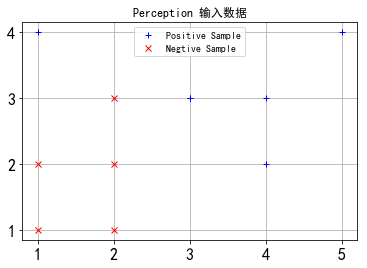
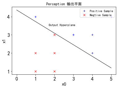
对于给定的一个数据集$T={(x_1,y_1),(x_2,y_2),…(x_n,y_n)}$,其中,$x_i \in X \subseteq R^n , y \in Y={-1, +1}, i=1,2,…,N$,如果存在某个超平面$S: w \cdot x+b = 0$,能将正负样例分到$S$两侧,则说明数据集$T$是线性可分的,那么接下来就是要求这个超平面$S$的表达式。

损失函数

数据集$T$中任意一个误分类点到这个超平面$S$的距离之和为:
$$\frac{1}{\Vert w \Vert}\sum_{x_i \in M}{\vert w \cdot x_i+b \vert}$$
其中$M$为误分类点的集合。如何去掉绝对值呢?我们注意到$y_i$的取值是有好处的。对于误分类点来说$y_i$的符号和$w \cdot x_i+b$相反。且$y_i$取值+1,-1。则我们可以将上式转换成:
$$- \frac{1}{\Vert w \Vert}\sum_{x_i \in M}{y_i (w \cdot x_i+b)}$$
确定损失函数时,不考虑$\frac{1}{\Vert w \Vert}$。

  • Q:感知机损失函数确定过程中的系数$\frac{1}{\Vert w \Vert}$,为什么可以忽略?
  • 1)感知机的损失函数时基于误分类的,$L2$范数项不会影响$y_i (w \cdot x_i+b)$的正负判断,所以$\frac{1}{\Vert w \Vert}$对感知机学习算法的中间过程可有可无
  • 2)$\frac{1}{\Vert w \Vert}$不影响感知机学习算法的最终结果,当所有输入被正确分类时,不存在误分类的点,此时损失函数为零,缺少此项并不会影响感知机损失函数的收敛
  • 3)我思考的是即使缺少这个项,损失函数也能对线性可分数据在有限次学习后正确分开。李航书上有证明。
  • 4)权重$w$是一个向量,$\frac{1}{\Vert w \Vert}$的大小不会影响向量的方向,确定超平面是通过确定法向量$w$和截距$b$来确定的,而的大对权重$w$的方向没有任何影响,所以可以固定$\frac{1}{\Vert w \Vert}$|为1或者不考虑。

算法步骤

输入:训练数据$T={(x_1,y_1),(x_2,y_2),…(x_n,y_n)}$,其中,$x_i \in X \subseteq R^n , y \in Y={-1, +1}, i=1,2,…,N$,;学习率$\eta(0<\eta<=1)$;
输出:$w,b$;感知机模型$f(x)=sign(w \cdot x+b)$。

  • 1)选取初值$w_0,b_0$
  • 2)在训练集中选取数据$(x_i,y_i)$
  • 3)如果$y_i (w \cdot x_i+b)<0$,$w \leftarrow w+ \eta y_ix_i;b \leftarrow b+ \eta y_i $
  • 4)转至 2),直至训练集中没有误分类点

代码实现

1
2
3
4
5
6
7
8
9
10
11
12
13
14
15
16
17
18
19
20
21
22
23
24
25
26
27
28
29
#初始化
import numpy as np
import random
import matplotlib as mpl
import matplotlib.pyplot as plt
datas = [[(1,2),-1],[(2,1),-1],[(2,2),-1],[(1,4),1],[(3,3),1],[(5,4),1],[(3, 3), 1], [(4, 3), 1], [(1, 1), -1],[(2, 3), -1], [(4, 2), 1]]

#数据展示
fig = plt.figure('Input Figure')
mpl.rcParams['xtick.labelsize'] = 16 # x轴的字体大小
mpl.rcParams['ytick.labelsize'] = 16
plt.rcParams['font.sans-serif']=['SimHei'] # 用来正常显示中文标签

xArr = np.array([x[0] for x in datas])
yArr = np.array([x[1] for x in datas])
xPlotx,xPlotx_,xPloty,xPloty_ = [],[],[],[]
for i in range(len(datas)):
y = yArr[i]
if y>0:
xPlotx.append(xArr[i][0])
xPloty.append(xArr[i][1])
else:
xPlotx_.append(xArr[i][0])
xPloty_.append(xArr[i][1])
plt.title('Perception 输入数据')
plt.grid(True)
pPlot1,pPlot2 = plt.plot(xPlotx,xPloty,'b+',xPlotx_,xPloty_,'rx')
plt.legend(handles = [pPlot1,pPlot2],labels=['Positive Sample','Negtive Sample'],loc='upper center')
plt.show()
output_1.png
output_1.png
1
2
3
4
5
6
7
8
9
10
11
12
13
14
15
16
17
18
19
20
21
22
23
24
25
26
27
28
29
30
31
32
#感知机算法
w = np.array([1, 1])
b = 3
eta = 0.5
while True:
num = 0
for i in range(len(datas)):
num = num + 1
x = xArr[i]
y = yArr[i]
z = y*(np.dot(w,x)+b)
if z <= 0:
w = w+eta*y*x
b = b+eta*y
num = 0 # 只要更新一次,强制令num=0,否则到最后一个数据不满足条件更新后,会直接跳出,而此时并不满足条件。
break
if num >= len(datas):
break
fig = plt.figure('Output Figure')
plt.title('Perception 输出平面')
x0 =np.linspace(0,5,100)
w0 = w[0]
w1 = w[1]
x1 = -(w0/w1)*x0-b/w1
plt.xlabel('x0',fontsize=15)
plt.ylabel('x1',fontsize=15)
plt.plot(x0,x1,'k', lw=1)
pPlot1,pPlot2 = plt.plot(xPlotx,xPloty,'b+',xPlotx_,xPloty_,'rx')
plt.legend(handles = [pPlot1,pPlot2],labels=['Positive Sample','Negtive Sample'],loc='upper right')
plt.annotate('Output Hyperplane',xy=(2.0,3.0),xytext=(1.7,3.5)) # 图形注释 # xy设置箭头尖的坐标,xytext设置注释内容显示的起始位置

plt.show()
output_2.png
output_2.png